
In the era of complex machine learning models, the need for transparency and understanding has never been greater.
As AI systems increasingly influence critical decisions in fields like finance, healthcare, and criminal justice, it’s crucial to be able to explain and interpret their outputs.
This post explores the concepts of model explainability and interpretability, using the Adult dataset (also known as the Census Income dataset) as a practical example.
You can find the complete code in my GitHub repository.
Explainability vs. Interpretability
While often used interchangeably, these terms have subtle differences:
Model explainability refers to the ability to describe the factors and the process by which a model makes its decisions.
Interpretability, on the other hand, is the degree to which a human can understand the cause of a decision made by a model.
Both concepts are critical, particularly in high-stakes applications such as finance, healthcare, and criminal justice, where understanding why a model made a particular decision is as important as the decision itself.
Trust: Users and stakeholders need to trust the model’s decisions.
Ethical Considerations: Transparent models help in identifying and mitigating biases.
Debugging: Understanding the model helps in identifying and fixing errors.
Regulatory Compliance: Many sectors require explainable AI for legal reasons.
Techniques for Model Explainability
1. SHAP (SHapley Additive exPlanations)
SHAP values provide a unified measure of feature importance that works across various model types.
2. LIME (Local Interpretable Model-agnostic Explanations)
LIME explains individual predictions by approximating the model locally with an interpretable model.
3. Partial Dependence Plots (PDP)
PDPs show the marginal effect of a feature on the predicted outcome.
4. Permutation Importance
This technique measures feature importance by randomly shuffling feature values and observing the impact on model performance.
Example: Adult Dataset
To illustrate model explainability and interpretability, let’s work with the Adult dataset, also known as the Census Income dataset.
This dataset contains demographic information about individuals and is commonly used to predict whether a person earns more than $50,000 a year.
1. Building the Model
For this example, we’ll train a Gradient Boosting model, known for its predictive power but often criticized for being a black-box model due to its complexity.
Gradient Boosting is an ensemble learning technique that combines multiple weak learners (typically decision trees) to create a strong predictive model. While this approach often leads to high accuracy, it can make the model difficult to interpret.
2. Results of Model Evaluation
| precision | recall | f1-score | |
| Class 0 (majority) | 0.88 | 0.95 | 0.91 |
| Class 1 (minority) | 0.80 | 0.61 | 0.69 |
| Weighted Av. | 0.86 | 0.86 | 0.86 |
The above classification report provides a detailed performance evaluation of the Gradient Boosting model on the test set.
Our Gradient Boosting Classifier, trained on the Census Income dataset, achieved an accuracy of 86% on the test set. This accuracy indicates that the model is robust in predicting whether an individual’s income exceeds $50,000 based on the provided features.
3. Model Explainability
To understand the underlying decision-making process of our model, we utilized several interpretability techniques, including SHAP (SHapley Additive exPlanations), Partial Dependence Plots (PDP), and LIME (Local Interpretable Model-agnostic Explanations).
These tools provided valuable insights into the key drivers of the model’s predictions:
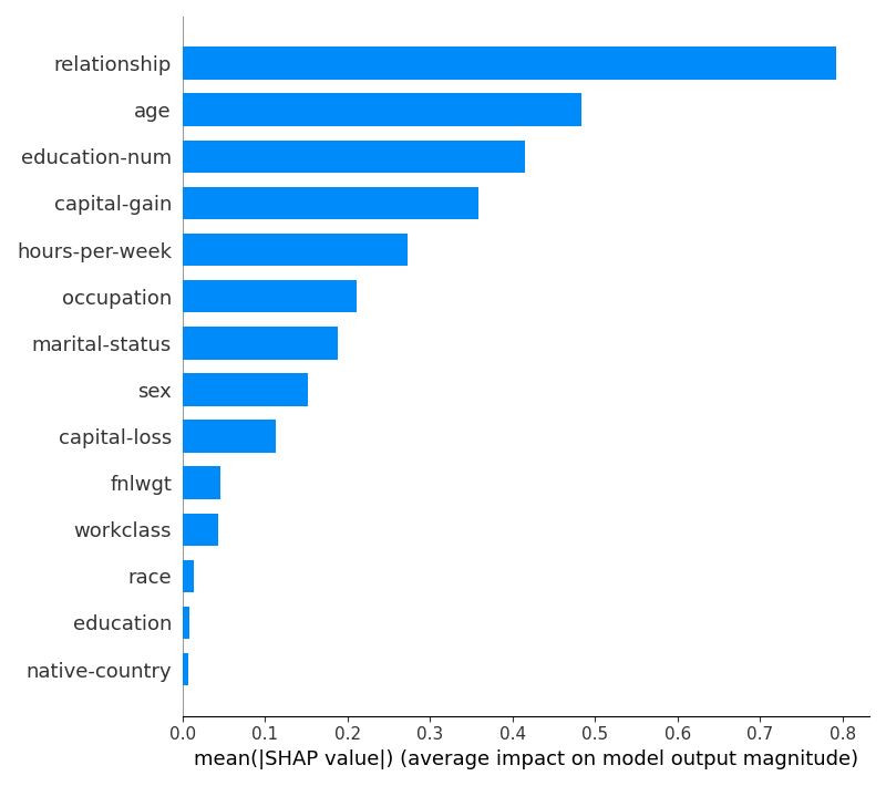
SHAP Summary Plot
The SHAP summary plot revealed that relationship status, age, and education level (measured by education-num) are the most influential features in determining income.
- Relationship status emerged as the top predictor, indicating significant variation in income levels based on marital and familial roles.
- Age and education-num followed closely, reflecting the expected correlation between more experience, higher education, and increased earning potential.
- Other notable features included capital-gain, hours-per-week, and occupation, all of which had moderate impacts on the model’s predictions.
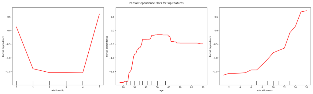
Partial Dependence Plots (PDP)
The PDPs provided a deeper look at how specific features influence predictions across the dataset.
- Relationship: there was a sharp decrease in the probability of earning >$50K for certain relationship statuses, highlighting the socioeconomic impact of marital and family roles.
- Age demonstrated a clear trend where income probability increases with age until it plateaus, suggesting that experience contributes positively to income, but only up to a certain point.
- Education-num (years of education) showed a strong positive correlation with income, emphasizing the value of higher education in boosting earning potential.
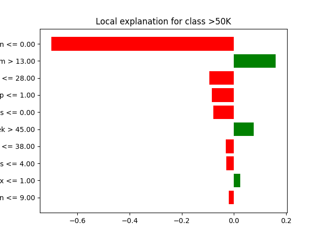
LIME Explanation
LIME was used to provide a local explanation for an individual prediction.
The explanation highlighted that for the specific instance analyzed, features such as relationship, education-num, and age had the most significant influence on predicting the likelihood of earning >$50K.
This local interpretability helps in understanding how the model arrives at decisions for individual cases, ensuring transparency in the model’s predictions.
Conclusion
The interpretability techniques applied in this analysis not only validated the performance of our Gradient Boosting Classifier but also provided transparency into the model’s decision-making process.
Understanding that features like relationship, age, and education are strong predictors of income can inform future enhancements to the model and guide policymakers in addressing income disparities.
Overall, these insights demonstrate the power of machine learning models when combined with interpretability techniques to yield both accurate and explainable results.