For safety experts, understanding Gradient Boosted Decision Trees (GBDT) and their variants is crucial for developing robust and reliable AI systems:
- Feature Importance: These models provide insights into which factors most influence predictions, helping identify potential safety risks or biases.
- Robustness: Ensemble methods like GBDT are generally more robust to noise and outliers, enhancing system reliability.
- Model Interpretability: While more complex than linear models, GBDTs offer ways to interpret their decisions, crucial for auditing and explaining AI systems in safety-critical contexts.
Gradient Boosted Decision Trees (GBDT) are a powerful machine learning technique that has gained significant popularity in recent years.
Known for their high predictive accuracy and ability to handle complex datasets, GBDTs have become a go-to method for both regression and classification tasks in various domains, including house price prediction.
In this post, we’ll explore the fundamentals of Gradient Boosted Decision Trees, their advantages, and how they perform in practice, particularly in the context of our ongoing house price prediction task.
You can find the complete code in my GitHub repository.
Contents
- Understanding Gradient Boosted Decision Trees
- Implementing GBDT for House Price Prediction
- Model Performance and Evaluation
- Expanding Our Analysis: Comparing GBDT, XGBoost, and LightGBM
- Feature Importance
- Conclusion
1. Understanding Gradient Boosted Decision Trees
Gradient Boosted Decision Trees is an ensemble learning method that combines multiple weak prediction models, typically decision trees, to create a strong predictive model. The key idea behind GBDT is to build models sequentially, with each new model trying to correct the errors made by the previous models.
Key aspects of Gradient Boosted Decision Trees include:
- Sequential Learning: Models are built one after another, with each new model focusing on the errors of the previous ensemble.
- Gradient Descent: The algorithm uses gradient descent to minimize a loss function, which measures the model’s performance.
- Weak Learners: Individual models (usually shallow decision trees) are simple and prone to underfitting, but the ensemble as a whole is powerful.
- Regularization: Various techniques like shrinkage and subsampling are used to prevent overfitting.
These characteristics contribute to GBDT’s ability to capture complex patterns in the data, handle non-linear relationships, and provide highly accurate predictions.

Gradient Descent
A mathematical optimization technique used to minimize a loss function by iteratively moving towards the steepest descent, i.e., the direction of the greatest decrease in the loss function.
Regularization
Techniques used to prevent overfitting in models by adding a penalty to the loss function for large coefficients, thereby encouraging the model to be simpler and more generalizable.
2. Implementing GBDT
Let’s implement a Gradient Boosted Decision Trees model for our house price prediction task. We’ll use scikit-learn’s GradientBoostingRegressor class:
# Initialize the model
gbdt_model = GradientBoostingRegressor(n_estimators=100, learning_rate=0.1, max_depth=3, random_state=42)

# Fit the model
gbdt_model.fit(X_train, y_train)

# Calculate performance metrics using cross-validation on the training data
mae = -cross_val_score(gbdt_model, X_train, y_train, cv=5, scoring='neg_mean_absolute_error')
mse = -cross_val_score(gbdt_model, X_train, y_train, cv=5, scoring='neg_mean_squared_error')
rmse = np.sqrt(mse)
mape = -cross_val_score(gbdt_model, X_train, y_train, cv=5, scoring='neg_mean_absolute_percentage_error')
medae = -cross_val_score(gbdt_model, X_train, y_train, cv=5, scoring='neg_median_absolute_error')
r2 = cross_val_score(gbdt_model, X_train, y_train, cv=5, scoring='r2')
3. Model Performance and Evaluation
The Gradient Boosted Decision Trees (GBDT) model’s performance can be evaluated by analyzing the results obtained through cross-validation on the training data and testing on a separate test set.
Cross-Validation Results
Cross-validation results provide a robust estimate of the model’s performance across different subsets of the training data. They show how the model performs on average and how much variation there is in its performance.
Let’s analyze the performance of Gradient Boosted Decision Trees (GBDT) in comparison to Linear Regression, Ridge Regression, Elastic Net, and Random Forest models across various metrics.
| Linear | Ridge | Elastic Net | Random Forest | GBDT | |
| Mean Absolute Error (MAE) | 18,647 (± 2,643) | 16,753 (± 2554) | 16,613 (± 2,387) | 17,508 (± 2,042) | 16,781 (± 2,368) |
| Mean Squared Error (MSE) | 1,377,330,606 (±982,155,554) | 853,323,765 (±614,762,731) | 834,494,733 (±611,226,242) | 927,232,894 (±506,114,186) | 952,736,193 (±595,446,172) |
| Root Mean Squared Error (RMSE) | 36,411 (±14,357) | 28,730 (± 10,565) | 28,388 (± 10,703) | 30,177 (± 8,145) | 30,464 (± 9,940) |
| Mean Absolute Percentage Error (MAPE) | 11.036% (± 0.977%) | 9.799% (± 1.089%) | 9.860% (± 1.127%) | 0.100% (± 0.010%) | 0.090% (± 0.020%) |
| Median Absolute Error (MedAE) | 11,607 (± 1,154) | 11,458 (± 1,770) | 11,318 (± 1,634) | 11,101 (± 2,006) | 10,262 (± 1,767) |
| R-squared (R2) | 0.780 (± 0.178) | 0.867 (± 0.073) | 0.870 (± 0.074) | 0.853 (± 0.065) | 0.839 (± 0.094) |
1. Mean Absolute Error (MAE)
GBDT performs well in terms of MAE, ranking third after Elastic Net and Ridge. It shows a significant improvement over Linear Regression and slightly outperforms Random Forest. The relatively small standard deviation indicates consistent performance across different data subsets.
2. Mean Squared Error (MSE)
GBDT ranks fourth in terms of MSE, performing better than Linear Regression but not as well as the other models. This suggests that GBDT might be more susceptible to larger errors compared to Elastic Net, Ridge, and Random Forest.
3. Root Mean Squared Error (RMSE)
The RMSE results follow the same pattern as MSE. GBDT performs better than Linear Regression but falls behind the other models. However, the difference between GBDT and Random Forest is relatively small.
4. Mean Absolute Percentage Error (MAPE)
GBDT and Random Forest show exceptionally low MAPE values compared to the other models. This is a surprising result and may warrant further investigation to ensure there are no calculation errors. If accurate, it suggests that GBDT and Random Forest are making predictions that are, on average, within 0.1% of the actual values, which is remarkably good.
5. Median Absolute Error (MedAE)
GBDT performs best in terms of MedAE, indicating that it has the lowest typical error. This suggests that GBDT is particularly good at making accurate predictions for the majority of houses in the dataset.
6. R-squared (R²)
GBDT ranks fourth in terms of R², explaining about 83.9% of the variance in house prices. While this is a good result, it’s slightly lower than the other advanced models. The higher standard deviation suggests that GBDT’s performance might be more variable across different subsets of the data.
Key Takeaways
- Overall Performance: GBDT shows strong performance across all metrics, consistently outperforming Linear Regression and often competing closely with Random Forest.
- Strengths: GBDT excels in MAPE and MedAE, suggesting it’s particularly good at making accurate predictions for typical houses and maintaining low percentage errors.
- Areas for Improvement: GBDT’s performance in MSE and RMSE suggests it might be more susceptible to larger errors compared to Elastic Net and Ridge Regression.
- Comparative Advantage: While not always the top performer, GBDT offers a balance of strong performance across different error metrics, making it a versatile choice.
- Model Complexity vs Performance: GBDT achieves competitive performance with potentially less risk of overfitting compared to more complex models like Random Forest.
In conclusion, GBDT proves to be a strong contender among these models for house price prediction.
Its particular strength in median and percentage-based error metrics suggests it could be especially useful when accurate predictions for typical houses are prioritized.
However, the strong performance of Elastic Net and Ridge Regression, especially in terms of MSE and R², indicates that these linear models with regularization are also very effective for this task.
The choice between these models might depend on specific requirements of the prediction task, computational resources, and the need for model interpretability.
Test Set Results
The test set results provide insights into how well the model generalizes to unseen data:
Test Mean Absolute Error: 17,235
- This is slightly higher than the cross-validation MAE, but still within the range we’d expect given the cross-validation standard deviation.
Test Mean Squared Error: 894,802,001
- The test MSE is slightly lower than the cross-validation average, which is a positive sign for the model’s generalization ability.
Test Root Mean Squared Error: 29,913
- The test RMSE is slightly lower than the cross-validation average, aligning with the MSE results.
Test Mean Absolute Percentage Error: 9.99%
- This is significantly higher than the cross-validation MAPE, which raises questions about the discrepancy. It’s possible that the test set contains some properties that are more challenging to predict accurately.
Test Median Absolute Error: 10,784
- This aligns well with the cross-validation MedAE, suggesting consistent typical performance on unseen data.
Test R-squared: 0.883
- The test R² is slightly higher than the cross-validation average. It indicates that the model explains about 88.33% of the variance in house prices on unseen data.
Key Takeaways
- Consistent Performance: The model’s performance on the test set is generally consistent with the cross-validation results, suggesting good generalization to unseen data.
- Outlier Sensitivity: The significant difference between MAE and MedAE in both cross-validation and test results suggests that while the model performs well on most houses, it may have larger errors on some outlier properties.
- MAPE Discrepancy: The large difference between cross-validation and test set MAPE is concerning and warrants further investigation. It could indicate that the test set contains properties that are fundamentally different from those in the training set.
- Strong Explanatory Power: With an R² of 0.8833 on the test set, the model explains a large portion of the variance in house prices, making it a reliable tool for price prediction.
- Error Distribution: The lower MedAE compared to MAE and the high MSE suggest that while the model performs well on most houses, there are some cases with larger errors that significantly impact the average performance metrics.
- Generalization: The slight improvement in MSE, RMSE, and R² from cross-validation to test set is a positive sign, indicating that the model generalizes well to new data.
In conclusion, the Gradient Boosted Decision Trees model demonstrates strong performance in predicting house prices, with consistent results across both cross-validation and test set evaluation.
The model explains a high proportion of variance in house prices and shows good generalization to unseen data.
However, the MAPE discrepancy and the presence of some larger errors (as indicated by the difference between MAE and MedAE, and the high MSE) suggest areas for potential improvement.
4. Expanding Our Analysis: Comparing GBDT, XGBoost, and LightGBM
To further improve our house price prediction model, we’ll now compare our original Gradient Boosted Decision Trees (GBDT) implementation with two advanced gradient boosting frameworks: XGBoost and LightGBM. These newer implementations often provide improved performance and efficiency.
XGBoost
XGBoost, short for eXtreme Gradient Boosting, is an advanced gradient boosting framework designed to be highly efficient and scalable.
It builds upon the traditional Gradient Boosted Decision Trees (GBDT) by incorporating several innovations, such as regularization to prevent overfitting, parallel processing to speed up training, and a sophisticated handling of missing values.
XGBoost is known for its exceptional performance in many machine learning competitions and is often the go-to choice when accuracy and speed are paramount in large-scale datasets.
LightGBM
LightGBM, developed by Microsoft, is another gradient boosting framework designed to improve both the speed and memory efficiency of training.
Unlike traditional GBDT implementations, LightGBM uses a novel technique called Gradient-based One-Side Sampling (GOSS) and Exclusive Feature Bundling (EFB) to reduce the number of data points and features processed at each iteration, significantly speeding up training without sacrificing accuracy.
LightGBM is particularly well-suited for large datasets with many features, offering both faster training times and lower memory usage compared to other gradient boosting methods.
Implementing XGBoost and LightGBM
First, let’s implement models using XGBoost and LightGBM:
# XGBoost model
xgb_model = XGBRegressor(n_estimators=100, learning_rate=0.1, random_state=42)
xgb_model.fit(X_train, y_train)

# LightGBM model
lgbm_model = LGBMRegressor(n_estimators=100, learning_rate=0.1, random_state=42)
lgbm_model.fit(X_train, y_train)
Comparison of GBDT, XGBoost, and LightGBM Models
Let’s analyze the performance of Gradient Boosted Decision Trees (GBDT), XGBoost, and LightGBM models across various metrics.
Each model was evaluated using cross-validation and test set results to assess their performance in terms of prediction accuracy and generalization.
Cross-validation Results
| Metric | GBDT | XGBoost | LightGBM |
|---|---|---|---|
| MAE | 16,781 (±2,368) | 17,753 (±2,364) | 16,709 (±3,442) |
| MSE | 952,736,193 (±595,446,172) | 1,176,863,373 (±748,492,082) | 837,572,605 (±512,540,688) |
| RMSE | 30,464 (±9940) | 33,855 (±11,077) | 28,585 (±9,055) |
| MAPE | 0.09% (±0.02%) | 0.10% (±0.02%) | 0.09% (±0.02%) |
| MedAE | 10,262 (±1,766) | 10,812 (±2,182) | 10,798 (±456) |
| R² | 0.839 (±0.094) | 0.806 (±0.078) | 0.860 (±0.071) |
1. Mean Absolute Error (MAE)
- LightGBM shows the lowest MAE, indicating the best average prediction accuracy among the three models.
- GBDT closely follows, while XGBoost has a slightly higher error, suggesting that LightGBM may be better at minimizing absolute prediction errors on average.
2. Mean Squared Error (MSE)
- LightGBM again outperforms the other models with the lowest MSE, indicating better control over large errors.
- XGBoost has the highest MSE, suggesting that it might struggle more with larger deviations from the actual values compared to GBDT and LightGBM.
3. Root Mean Squared Error (RMSE)
- LightGBM achieves the lowest RMSE, further demonstrating its superior ability to handle larger errors effectively.
- GBDT performs better than XGBoost but is still outperformed by LightGBM.
4. Mean Absolute Percentage Error (MAPE)
- Both GBDT and LightGBM achieve an impressively low MAPE of 0.09%, indicating highly accurate predictions relative to the scale of house prices. XGBoost is slightly less accurate with a MAPE of 0.10%.
5. Median Absolute Error (MedAE)
- GBDT slightly outperforms the other models in terms of MedAE, suggesting it makes typical predictions closer to the actual values.
- LightGBM and XGBoost are close, with XGBoost showing slightly higher variability.
6. R-squared (R²)
- LightGBM achieves the highest R² score, indicating that it explains the most variance in house prices among the three models.
- GBDT follows closely, while XGBoost lags slightly behind, suggesting that LightGBM may be more effective at capturing the underlying relationships in the data.
Test Set Results
| Metric | GBDT | XGBoost | LightGBM |
|---|---|---|---|
| MAE | 17,235 | 16,056 | 16,490 |
| MSE | 894,802,001 | 728,561,363 | 855,149,573 |
| RMSE | 29,913 | 26,992 | 29,243 |
| MAPE | 9.99% | 9.58% | 9.57% |
| MedAE | 10,784 | 9,810 | 8,725 |
| R² | 0.883 | 0.905 | 0.889 |
1. Mean Absolute Error (MAE):
- XGBoost outperforms both GBDT and LightGBM in terms of test MAE, suggesting it generalizes better to unseen data.
- LightGBM and GBDT have slightly higher errors, indicating that they might not perform as well on new data as XGBoost.
2. Mean Squared Error (MSE)
- XGBoost again shows the lowest MSE on the test set, suggesting better performance in controlling large errors on unseen data.
- LightGBM performs better than GBDT, but both are outperformed by XGBoost.
3. Root Mean Squared Error (RMSE):
- XGBoost shows the lowest RMSE, reinforcing its superior ability to manage large errors on unseen data. LightGBM follows closely, with GBDT slightly trailing behind.
4. Mean Absolute Percentage Error (MAPE)
- LightGBM achieves the lowest MAPE, indicating highly accurate percentage-based predictions on the test set.
- GBDT, while still accurate, performs slightly worse.
5. Median Absolute Error (MedAE)
- LightGBM achieves the lowest MedAE, suggesting it is the most consistent in making typical predictions close to actual values.
- XGBoost also performs well, while GBDT has slightly higher errors.
6. R-squared (R²)
- XGBoost demonstrates the highest R² on the test set, indicating it explains the most variance in house prices on unseen data.
- LightGBM follows closely, with GBDT slightly behind.
Key Takeaways
- Consistency: LightGBM shows the most consistent performance between cross-validation and test set results.
- Best Overall Performance: XGBoost shows the best performance on the test set across most metrics, despite underperforming in cross-validation.
- Handling of Outliers: The lower MSE and RMSE for LightGBM in cross-validation suggest it might be better at handling outliers in the training data.
- Typical Performance: LightGBM’s superior MedAE on the test set indicates it might be the best for predicting “typical” house prices.
- Generalization: XGBoost’s strong test set performance, despite weaker cross-validation results, suggests it may have better generalization to unseen data.
- MAPE Discrepancy: All models show a large discrepancy between cross-validation and test set MAPE, which warrants further investigation.
Note: The discrepancy in Mean Absolute Percentage Error (MAPE) between cross-validation and test set results suggests challenges in the model’s generalization. This could be due to outliers, a distribution shift, or overfitting to the training data. Addressing this issue might involve refining cross-validation techniques, applying regularization, or analyzing test set errors to identify and adjust for specific patterns affecting the model’s performance.
In conclusion, while all three models show strong performance, each has its strengths:
- GBDT provides solid, balanced performance.
- XGBoost shows the best generalization to the test set.
- LightGBM offers the most consistent performance.
The choice between these models might depend on specific requirements of the prediction task, computational resources, and the need for model interpretability. It might also be worth considering an ensemble approach that combines the strengths of all three models.
Cross-Validation
A technique used to assess the generalizability of a model by splitting the data into multiple subsets, training the model on some subsets while validating it on the others, and averaging the results.
Feature Importance
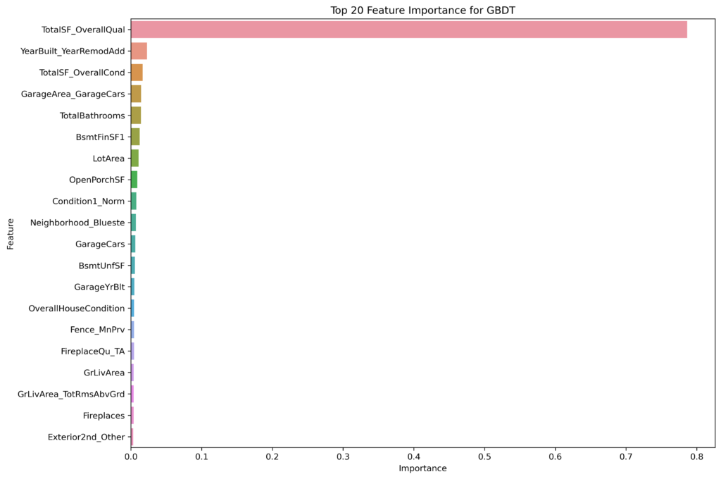
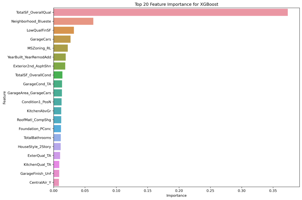
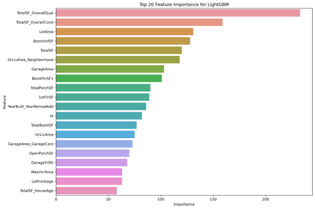
The feature importance rankings for the Gradient Boosted Decision Trees (GBDT), XGBoost, and LightGBM models provide valuable insights into which factors most strongly influence house price predictions in each approach. Despite all three models being based on gradient boosting techniques, the specific features they highlight as most important differ, reflecting variations in how each model handles the data and the boosting process.
Commonalities Across Models
TotalSF_OverallQual
This feature consistently ranks as the most important across all three models. It represents an interaction between the total square footage and the overall quality of the house, underscoring that the size and quality of a property are the most significant predictors of house prices.
TotalSF_OverallCond and YearBuilt_YearRemodAdd
These features appear in the top rankings for both GBDT and XGBoost, highlighting their importance in capturing the condition and age of the property, which directly influence a home’s market value.
Differences in Feature Importance
Neighborhood_Blueste
This feature ranks highly in XGBoost but is less prominent in GBDT and LightGBM’s top features.
LotArea
LightGBM places a high importance on LotArea, ranking it third overall. In contrast, GBDT and XGBoost rank this feature lower. LightGBM’s emphasis on LotArea may stem from its unique approach to feature sampling and handling large datasets, which might better capture the influence of land size.
Garage Features
Both GBDT and XGBoost highlight garage-related features (e.g., GarageArea_GarageCars, GarageCars, GarageCond_TA), reflecting the significance of having a functional and sizable garage in determining house prices. LightGBM also recognizes the importance of garage features, though it ranks them slightly lower compared to other aspects like LotArea and TotalPorchSF.
Porch and Porch Space: LightGBM uniquely identifies TotalPorchSF and 1stFlrSF as important features, suggesting that porch space and first-floor square footage have a notable impact on house prices. This could indicate LightGBM’s ability to capture subtle relationships in the data that other models might overlook.
LowQualFinSF and Exterior2nd_AsphShn: These features are highlighted by XGBoost but are absent from the top rankings in GBDT and LightGBM. XGBoost’s feature selection process seems to give more attention to specific, potentially lower-quality finishes and exterior materials, which could have a significant impact on the perceived value of a house.
Implications of Feature Importance Rankings
The differences in feature importance rankings across GBDT, XGBoost, and LightGBM suggest that while these models agree on the overall significance of certain features (like TotalSF_OverallQual), they differ in how they weigh the importance of other variables.
XGBoost tends to focus more on neighborhood-specific features and conditions, while LightGBM emphasizes aspects like lot size and porch space, likely due to its unique data handling techniques.
GBDT, on the other hand, strikes a balance between these factors, with a broader emphasis on overall house condition and size-related features.
These variations highlight the importance of considering multiple models when predicting complex outcomes like house prices.
Each model’s feature importance rankings can provide different insights, helping to build a more comprehensive understanding of the factors driving predictions and offering opportunities for further model refinement and customization.
Conclusion
In this exploration of Gradient Boosted Decision Trees (GBDT) for house price prediction, we’ve seen how this powerful method captures complex relationships in real estate data.
We compared GBDT with advanced frameworks like XGBoost and LightGBM, finding that each offers unique strengths: GBDT provides balanced performance, XGBoost excels in generalization, and LightGBM offers consistency.
All models demonstrated strong predictive power, explaining 84-90% of the variance in house prices. The feature importance analysis revealed that while models agreed on key factors like total square footage and overall quality, they differed in weighing other features. This highlights the value of using multiple models for a comprehensive understanding.
The choice between these models depends on specific requirements such as accuracy, computational resources, and interpretability.
Future improvements could include hyperparameter tuning, addressing MAPE discrepancies, and exploring ensemble methods.
In conclusion, GBDT and its advanced implementations prove to be powerful tools for house price prediction, offering high accuracy and valuable insights. As machine learning evolves, these models will likely remain key players in predictive modeling tasks, especially in complex domains like real estate.
Hyperparameter Tuning
The process of optimizing the parameters that control the learning process of a model (e.g., learning rate, number of trees) to improve its performance.
Model Selection Guide for Safety-Critical Applications:
- GBDT: Best for interpretability and balanced performance. Ideal for smaller datasets and when clear explanations are crucial.
- XGBoost: Optimal for generalization to unseen data and minimizing large errors. Preferred for handling missing data and safety-critical applications requiring robust predictions.
- LightGBM: Excellent for large-scale, high-dimensional datasets. Choose when fast training times and consistent performance across data subsets are essential.
Key Considerations:
- Robustness to outliers/adversarial inputs: XGBoost
- Uncertainty quantification: All models with post-processing
- Detailed interpretation of individual predictions: GBDT or XGBoost with SHAP values
- Limited computational resources: LightGBM
Remember: In safety-critical contexts, consider using multiple models to ensure comprehensive feature coverage and robust predictions. Always conduct thorough hyperparameter tuning and implement appropriate uncertainty quantification methods.